
That tempting big salary might not be all it seems. That’s because places where pay is high tend to be more expensive. Jobs offer a premium in the Bay Area, Boston, Washington and New York. But those extra dollars go right back out to pay for higher rents and pricier meals. Adjusted for living costs, salaries are highest not in the big coastal metros, but in less attention-getting locales like Brownsville, TX, Kingsport, TN, and Huntington, WV.
But before you reserve that one-way U-Haul to take you to Kingsport, know this: places where adjusted salaries are higher often serve up other challenges. They tend to have higher unemployment today and are projected to have slower job growth. If you want it all — high adjusted salaries, low unemployment today and good future prospects — look instead at Duluth, MN, Wilmington, NC, and Lubbock, TX.
And let’s be realistic. You might not want to trek across the country, far from family, friends or weather you love, to a place where jobs in your field are scarce. That’s fine. You can probably move somewhere not too far away with a similar mix of jobs and boost your standard of living at the same time — for example, by relocating from Tampa to Birmingham or from San Diego to Sacramento. Most places have relatively close-by sister cities where adjusted salaries are at least a bit higher.
Where adjusted salaries are highest
Before adjusting for cost of living, America’s highest salaries are in metro San Jose, the heart of Silicon Valley. To see this, we calculated the average salary for all Indeed job postings between July 2017 and June 2018 that included information on annual salaries, accounting for differences in the local job mix. For the same occupations, salaries are on average 19% higher in San Francisco than in San Antonio and 18% higher in Boston than in Cleveland.
But San Antonio and Cleveland are cheaper than San Francisco and Boston. Housing costs less, as do other goods and services. Adjusted for living costs, salaries are actually 11% higher in San Antonio than in San Francisco and 5% higher in Cleveland than in Boston.
Among the 185 US metropolitan areas with at least 250,000 people, salaries adjusted for living costs are highest in Brownsville-Harlingen, TX, Kingsport-Bristol-Bristol, TN-VA, and Huntington-Ashland, WV-KY-OH. Of the top 10, only Birmingham-Hoover has more than a million people. Larger metros have higher unadjusted salaries, but much higher living costs than smaller metros. As a result, adjusted salaries tend to be higher in smaller metros. The million-plus metros with the highest adjusted salaries are Birmingham-Hoover, Cincinnati, Cleveland, Memphis, and San Antonio.
[table id=31 Autocomplete=0 center=1,2 search=”Search by Metro”/]
Adjusted salaries are lowest in Honolulu, Santa Cruz, CA, Oxnard, CA, Miami, and New York. It’s no coincidence that these are all desirable spots for weather, recreation or lifestyle. Many people are willing to give up some income or pay more for housing to live in places with such amenities. In fact, classical urban economics models interpret low adjusted salaries as an indicator of high local quality of life. That’s something to consider before moving someplace where adjusted salaries are high, but amenities are fewer.
Not just money: higher salaries and opportunities today and tomorrow
Even if you’re only considering economic factors when choosing a new hometown, don’t stop at adjusted salaries. Unless you’ve already got a secure job in hand, you should consider the ease of finding a job today and the odds of having one in the future.
Strikingly, places with high adjusted salaries fare poorly both in terms of job prospects today and tomorrow. First, local unemployment rates tend to be higher in metros with higher adjusted salaries. In June 2018, unemployment was more than 8% in Merced and nearly 7% in Brownsville-Harlingen, TX — well above the 4.2% national rate without seasonal adjustment.
Second, projected job growth is lower in metros with higher adjusted salaries. Among the top 10 metros for adjusted salaries, projected job growth based on local occupation mix is particularly low in Kingsport-Bristol-Bristol, TN-VA, Spartanburg, SC, and Hickory-Lenoir-Morganton, NC. Projected job growth is highest in large coastal metros, which tend to be expensive and have lower adjusted salaries.
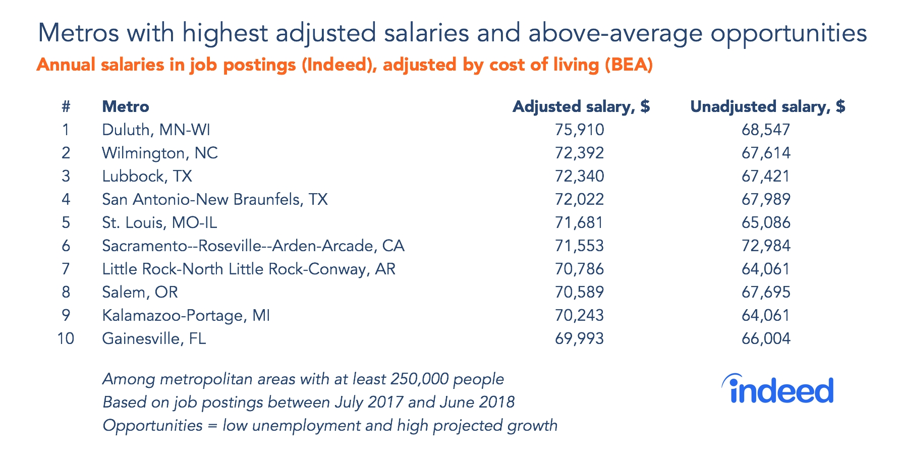
So let’s take another look at the top metros for adjusted salaries, excluding those that are worse than average for either current unemployment or projected job growth. None of the overall top 10 make the cut. The top 10 metros for adjusted salaries with better-than-average unemployment today and future growth prospects comprise an entirely different list. Duluth, MN-WI, Wilmington, NC, and Lubbock, TX, offer the highest cost-adjusted pay as well as good job opportunities today and tomorrow. Several large metros are also on this list.
Higher salaries without too much change
Much as we love top 10 lists, we know that your number one might not be my number one. For instance, St. Louis may have high adjusted salaries, low unemployment, and strong future growth, but it has relatively few job postings for economists — and I’m not looking to make a career change. And Duluth might be a tough sell for someone used to mild California winters.
Still, there’s often another local market out there with higher adjusted salaries and a similar job mix that’s not too far away. To flesh that out, we looked for the biggest differences in adjusted salaries for pairs of metros that are less than 500 miles apart and have at least a 75% overlap in their mix of job postings. At the top: Birmingham’s adjusted salaries are 22% higher than Tampa’s, and Sacramento’s are 21% above Oxnard-Thousand Oaks-Ventura’s.
[table id=30 Autocomplete=0,1 center=2 search=”Search by Metro”/]
These are moves that get you a higher standard of living and similar job opportunities — all just a short flight or day’s drive away. Those adjusted-salary differences might sound small relative to the gap between extremes: Brownsville’s adjusted salaries are 51% higher than Honolulu’s, and Kingsport’s are 37% higher than those in Santa Cruz. But you’d need to move a long distance to a very different labor market — and hope to find a job that fits you — in order to claim that higher standard of living. All else equal, a higher adjusted salary is better than a lower one. But in job hunting — like so many other things — all else is never equal.
Methodology
Salary data are from all job postings with annual salaries on Indeed between July 2017 and June 2018. Unadjusted average salaries are based on weighted median deviations across occupations, which accounts for the different mix of job titles across metros in order to make an apples-to-apples comparison of unadjusted salaries.
Local cost-of-living data are from the U.S. Bureau of Economic Analysis regional price parities for 2016, released May 2018. These cost-of-living data reflect local differences in the price of housing, other services, and physical goods. Unemployment data are from the Bureau of Labor Statistics and are not seasonally adjusted, unlike the published headline rate. Projected job growth is from Indeed’s analysis of Bureau of Labor Statistics projections.
All 185 U.S. metropolitan areas with at least 250,000 people are included in the rankings.
Distances between metros are great-circle distances between population-weighted metro centroids, which tend to be a bit shorter than actual driving distances.
Unadjusted and adjusted salary data in this blogpost should not be compared with salary data from last year’s blogpost on this topic. The occupational composition of job postings with annual salaries changes over time. Our methodology adjusts for differences in occupational composition across metros at a point in time, but not for differences in occupational composition over time.